where $\boldsymbol{q}_t,\boldsymbol{k}_i,\boldsymbol{v}_i\in\mathbb{R}^d$; for notational brevity we absorb the scaling factor $1/\sqrt{d}$ into $\boldsymbol{q}$. Every query has to take inner products with all $L$ keys and then normalize, so the overall complexity is quadratic, $\mathcal{O}(L^2)$. This is already very expensive in the long-context regime of LLMs, and for video generation or high-resolution image generation it only makes things worse. As an example: suppose we want to generate a 720×1280, 24 fps, one-minute video, and the VAE compression ratio is $(4,16,16)$ (time × height × width); then the latent sequence has
about 1.3 million tokens. At this length, quadratic-complexity attention is essentially unacceptable.
To make the derivations below easier to follow, let me fix the notation for the whole post: the sequence length is $L$ and the head dimension is $d$; vectors are column vectors by default, $\boldsymbol{q}\cdot\boldsymbol{k}$ denotes the inner product, and $\boldsymbol{v}\boldsymbol{k}^{\top}$ denotes the outer product (a $d\times d$ matrix); tokens are cut in order into blocks of size $B$, with the $j$-th block denoted $\mathcal{B}_j$, and the mean (centroid) of the keys within a block denoted $\bar{\boldsymbol{k}}_j=\frac{1}{B}\sum_{i\in\mathcal{B}_j}\boldsymbol{k}_i$; for a query $\boldsymbol{q}_t$, the set of selected top-K blocks is denoted $\mathcal{S}_t$ and the unselected ones $\mathcal{U}_t$.
Sparse Attention
In recent years there has been a great deal of work on sparse attention. The most emblematic examples include Kimi’s MoBA and DeepSeek-V3.2’s DSA. Not coincidentally, there is also plenty of similar work in video generation, such as VSA.
An empirical foundation of sparse attention is that transformer attention matrices are markedly sparse: at most positions the attention weight is very low. So the core idea of sparse attention is to cheaply estimate which positions contribute little to attention, discard them outright, and compute exact attention only at the top-K positions estimated to contribute most, thereby reducing computation. Concretely, in a few representative works:
DSA first scores with a lightning indexer that has few heads and can run in FP8: $I_{t,s}=\sum_{j=1}^{H^I} w_{t,j}\,\mathrm{ReLU}\big(\boldsymbol{q}^{I}_{t,j}\cdot\boldsymbol{k}^{I}_{s}\big)$, and then each query keeps only the top-K highest-scoring tokens (K = 2048) for exact attention.
MoBA splits tokens into blocks and uses the mean of the keys within a block as that block’s “representative” for scoring: $s_{t,j}=\boldsymbol{q}_t\cdot\bar{\boldsymbol{k}}_j$, and each query selects the top-K blocks.
VSA partitions video tokens into 3D blocks (cubes), mean-pools each cube to obtain coarse-grained $\boldsymbol{q},\boldsymbol{k}$, first runs a coarse cube-level attention to select the top-K cubes, and then performs fine-grained attention only within the selected cubes.
As we can see, the core of sparse attention is to cheaply estimate the top-K, compute exact softmax attention only at the top-K positions, and discard all the rest. This certainly brings the computational complexity down (in LLMs the top-K is typically on the order of 2048; in video generation one can usually reach around 5% or 10% sparsity). However, the information at the vast majority of positions is simply thrown away, which in my view is somewhat wasteful and not precise enough: those “long-tail” positions with low weights but enormous count add up to a contribution that is actually far from negligible.
Linear Attention
Linear attention has many variants and interpretations. In my view, the essence of linear attention is to approximate softmax attention. The most classic approach (Katharopoulos et al., 2020) picks a feature map satisfying $\phi(\cdot)\ge 0$ and replaces the exponential similarity with a kernel function: $\phi(\boldsymbol{q})\cdot\phi(\boldsymbol{k})\sim \exp(\boldsymbol{q}\cdot\boldsymbol{k})$ (a common choice being $\phi(x)=\mathrm{elu}(x)+1$). Substituting back into attention and using the associativity of multiplication to swap the order of summation yields vanilla linear attention:
The terms in parentheses, $\sum_i \boldsymbol{v}_i\phi(\boldsymbol{k}_i)^{\top}\in\mathbb{R}^{d\times d}$ and $\sum_i\phi(\boldsymbol{k}_i)\in\mathbb{R}^{d}$, are both query-independent and can be computed once (in the causal setting they become an RNN state recurrence), so the complexity drops from $\mathcal{O}(L^2)$ to $\mathcal{O}(L)$.
In fact, as also explained in Su Jianlin’s blog post, directly Taylor-expanding softmax attention likewise yields linear attention, and it is more direct than “first approximate $\exp(\boldsymbol{q}\cdot\boldsymbol{k})$ and then normalize”. Concretely, write the logits vector as $\boldsymbol{x}=(\boldsymbol{q}\cdot\boldsymbol{k}_1,\cdots,\boldsymbol{q}\cdot\boldsymbol{k}_L)$ and Taylor-expand around its mean $\bar{\boldsymbol{x}}$; the first-order truncation gives
The intuition behind this expression is quite elegant: the mean $\bar{\boldsymbol{k}}$ serves as the “baseline” of attention — tokens whose similarity with the query is above the mean get their weights increased, and those below the mean get them decreased. Plugging this back into $\boldsymbol{o}=\sum_i a_i\boldsymbol{v}_i$ and simplifying gives
which is exactly a (de-centered version of) vanilla linear attention.
Moreover, in a follow-up blog post, the well-known Gated DeltaNet (the KDA used in the recent Kimi K3 is a GDN variant that debuted in Kimi Linear) can also be derived via the same linearized approximation. Let me briefly paraphrase the idea. Fixing the query $\boldsymbol{q}$, the output of causal attention actually satisfies an exact recurrence:
The increment $\boldsymbol{v}_t-\boldsymbol{o}_{t-1}$ is “new observation minus old prediction”, already faintly resembling the delta rule. Next, one only needs to apply the first-order Taylor expansion above to the diagonal element $a_{t,t}$, i.e. $a_{t,t}\approx\frac{1}{t}\big(1+\boldsymbol{q}\cdot(\boldsymbol{k}_t-\bar{\boldsymbol{k}}_t)\big)$ (approximating only the diagonal rather than all of $a_{t,i}$, a much lighter approximation burden), then posit a solution of the form $\boldsymbol{o}_t\approx\boldsymbol{A}_t\boldsymbol{q}+\bar{\boldsymbol{v}}_t$, and, following a “minimum-error principle”, replace the residual $\boldsymbol{q}$ in the recurrence with $\boldsymbol{k}_t-\bar{\boldsymbol{k}}_t$, which yields
Comparing with GDN’s standard form $\boldsymbol{S}_t=\boldsymbol{S}_{t-1}\,\alpha_t(\boldsymbol{I}-\beta_t\boldsymbol{k}_t\boldsymbol{k}_t^{\top})+\beta_t\boldsymbol{v}_t\boldsymbol{k}_t^{\top}$, both the gating term $\alpha_t$ and the delta rule term emerge naturally. In other words, everything from vanilla linear attention to GDN can be unified under the single perspective of “linearized approximations of softmax attention”.
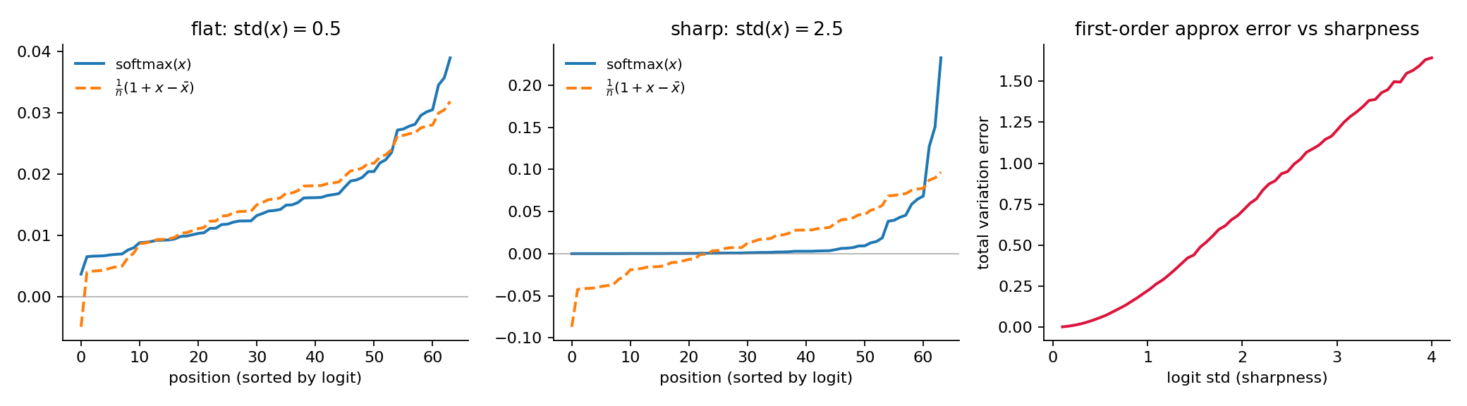
The complexity of linear attention is of course $\mathcal{O}(L)$ — very cheap. But precisely because its essence is an approximation of softmax attention, it necessarily incurs a loss. And from the Taylor-expansion viewpoint, the source of this loss is crystal clear: the first-order truncation discards the second- and higher-order terms in $\boldsymbol{y}=\boldsymbol{x}-\bar{\boldsymbol{x}}$, whose magnitude is governed by how far the logits deviate from their mean (higher-order moments like $\overline{\boldsymbol{y}^2}$). In other words, the sharper the original softmax attention distribution (the larger the logits variance), the larger the error of the linear approximation; whereas in regions where the distribution is flat, the linear approximation is quite accurate. The figure below shows a toy example: when the logits are flat, the first-order approximation hugs the true softmax distribution almost exactly; once the distribution becomes sharp, the approximation severely underestimates the peaks and even goes negative in the tails, with the total error growing rapidly with the standard deviation of the logits.
linear approx toy example
Sparse Linear Attention
Now put the two side by side, and you will find they are exactly complementary:
Linear attention can approximate the entire attention, but its error is large where the distribution is sharp (i.e., precisely where the top-K lives);
Sparse attention is exact softmax attention at the top-K positions, but it throws away the entire flat region, which makes up the vast majority — and the flat region is exactly where the linear approximation shines.
A natural idea is therefore to combine them: perform sparse softmax attention in the top-K region, and approximate everything else with linear attention. SLA (Sparse–Linear Attention) does exactly this. Concretely, it also estimates block-level attention weights via block-wise averaging, $P_c=\mathrm{Softmax}\big(\mathrm{pool}(\boldsymbol{Q})\,\mathrm{pool}(\boldsymbol{K})^{\top}\big)$, and accordingly divides blocks into three classes: the top 5% critical blocks go through exact block-sparse softmax attention, the bottom 10% are skipped outright, and the roughly 85% “marginal blocks” in the middle go through linear attention; finally the two parts are added together. However, the two parts are computed separately — that is, each has its own independent softmax normalization denominator:
Each branch normalizes its own weights to sum to 1, so adding them directly would skew the distribution; SLA therefore needs to introduce an extra learnable projection to compensate:
Clearly, this combination leaves a gap in approximating full softmax attention and cannot be training-free: SLA must fine-tune the model (fortunately the cost is modest — in the paper, only 2000 fine-tuning steps on Wan2.1-1.3B suffice to match full attention’s generation quality at 95% sparsity, with about 2.2× end-to-end speedup).
Then PISA (Piecewise Sparse Attention) proposed a natural improvement: rather than computing two attentions separately and learning a projection to stitch them together, why not directly split the same softmax attention into two parts, and linearize the non-top-K region via Taylor expansion? Write the output in numerator/denominator form $\boldsymbol{o}_t=\mathcal{N}_t/\mathcal{D}_t$, split both according to selected/unselected, and for each unselected block $j\in\mathcal{U}_t$, expand the exponential around the block centroid $\bar{\boldsymbol{k}}_j$:
i.e., a zeroth-plus-first-order Taylor expansion. Look at the denominator first: since the within-block deviations sum to zero ($\sum_{i\in\mathcal{B}_j}(\boldsymbol{k}_i-\bar{\boldsymbol{k}}_j)=\boldsymbol{0}$), the first-order term cancels exactly in the denominator, leaving only
In other words, each unselected block is compressed into a “virtual token” with weight $B\cdot\alpha_{t,j}$. The numerator, in turn, consists of three parts — the exact term, the zeroth-order term, and the first-order correction:
where $\boldsymbol{H}_j=\sum_{i\in\mathcal{B}_j}\boldsymbol{v}_i(\boldsymbol{k}_i-\bar{\boldsymbol{k}}_j)^{\top}$ is the first-order key–value cross statistic within a block. To make the first-order term strictly linear in complexity as well, PISA further replaces the per-block $\boldsymbol{H}_j$ with the average over all blocks, $\bar{\boldsymbol{H}}=\frac{B}{L}\sum_j\boldsymbol{H}_j$, so the first-order correction simplifies to $\big(\sum_{j\in\mathcal{U}_t}\alpha_{t,j}\big)\bar{\boldsymbol{H}}\,\boldsymbol{q}_t$, and all query-independent statistics can be precomputed.
Comparing with SLA, the key difference is immediately obvious: PISA’s exact branch and approximate branch share the same softmax denominator $\mathcal{D}_t$, so the two parts naturally live in the same normalization scheme — there is no distribution mismatch, and hence no need for an extra projection layer to stitch them together. Note that PISA’s method is by no means restricted to being training-free — the original paper only ran training-free experiments (on models such as Wan2.1 and HunyuanVideo, VBench is essentially lossless at 87.5% sparsity with about 2× speedup), which in my view precisely demonstrates how accurate its approximation of softmax attention is: without touching the model at all, it can be dropped in as a replacement for full attention.
Looking back, the thread is remarkably coherent: sparse attention says “positions with small weights don’t matter — throw them away”; linear attention says “the entire attention can be linearly approximated”; and sparse linear attention says: keep exact computation where the distribution is sharp, and approximate via Taylor expansion where the distribution is flat, upgrading “discard” to “approximate” — letting each of the two methods patch exactly the other’s weakness.
Going Further: Adding the Second-Order Term (PWT)
Scrutinize PISA’s expansion and you will notice an “asymmetry”: the numerator is taken to first order, while the denominator has only the zeroth order — of course this is not an omission; as derived above, the first-order term cancels exactly in the denominator because $\sum_{i\in\mathcal{B}_j}(\boldsymbol{k}_i-\bar{\boldsymbol{k}}_j)=\boldsymbol{0}$. But this is exactly what tells us: the denominator’s next non-zero correction lives at second order. And following the expansion of LogSumExp in Su Jianlin’s blog post, this second-order term has a very clean closed form. So I made a natural extension: complete PISA’s block-mass estimate up to second order, referred to below as PWT (Piecewise-Taylor).
The derivation takes only two lines. Write the true mass of an unselected block $j\in\mathcal{U}_t$ as the zeroth order times an average factor, let $y_{t,i}=\boldsymbol{q}_t\cdot(\boldsymbol{k}_i-\bar{\boldsymbol{k}}_j)$ (zero mean within the block), and Taylor-expand to second order:
which is precisely the covariance matrix of the keys within the block — the concrete, block-wise form of the second-order term $\overline{\boldsymbol{y}^2}/2$ in Su’s $\mathrm{logsumexp}$ expansion. Note that $w_{t,j}\ge 0$: by Jensen’s inequality, $\frac{1}{B}\sum_i e^{y_i}\ge e^{\bar{y}}=1$, which means the zeroth-order approximation systematically underestimates the block mass — the larger the within-block variance, the harsher the underestimate — and the second-order term corrects it in exactly the right direction. In the implementation we write $1+w$ as $e^{w}$ (equivalent for small $w$), so that it adds directly onto the virtual token’s logit — the virtual token’s weight goes from $B\,e^{\boldsymbol{q}_t\cdot\bar{\boldsymbol{k}}_j}$ to $B\,e^{\boldsymbol{q}_t\cdot\bar{\boldsymbol{k}}_j+w_{t,j}}$ — and the numerator’s zeroth-order term, the first-order correction’s weight, and the denominator all share the same corrected logit, so normalization stays consistent automatically, and not a single line of the online softmax pipeline needs to change.
The remaining question is the cost of $w_{t,j}$: computing $\boldsymbol{q}^{\top}\boldsymbol{C}_j\boldsymbol{q}$ per query per block is an $\mathcal{O}(d^2)$ expense. Here we apply two steps of cheapening: first take the diagonal approximation $\boldsymbol{q}^{\top}\boldsymbol{C}_j\boldsymbol{q}\approx\sum_{c} q_c^2\,\sigma_{j,c}^2$ (where $\sigma_{j,c}^2$ is the within-block variance of the $c$-th dimension), then pool $q^2$ along the query blocks. There is an easy pitfall here: the pooling must use $\overline{\boldsymbol{q}^2}$ (square first, then average) rather than $\bar{\boldsymbol{q}}^2$ (average first, then square) — the latter wipes out all the variance within the query block, and accuracy regresses noticeably. With this, $w$ degenerates into a small [query block × key block] matrix that, just like $\bar{\boldsymbol{k}}_j,\boldsymbol{H}_j$, can be computed once before entering the kernel; inside the kernel it is merely one broadcast addition — nearly zero extra overhead compared with PISA. We measured that this “diagonal + pooled” version has almost identical approximation error to computing $w$ exactly row by row, whereas the latter makes the kernel nearly twice as slow — the gains from the Taylor expansion lie entirely in this second-order statistic itself; going as fine-grained as per-row simply isn’t worth it.
Incidentally, the second-order term also gives the top-K routing a more principled interpretation: a block’s truncation error is roughly proportional to “mass × within-block heterogeneity”, so the score can be taken directly as $\log\big(B\,e^{\boldsymbol{q}\cdot\bar{\boldsymbol{k}}_j+w_j}\big)+\log\lVert\boldsymbol{H}_j\rVert$ — blocks with large mass or where the Taylor expansion fails (large variance) go into the exact branch. The covariance-aware block-selection heuristic in the original PISA paper is, from the expansion viewpoint, simply “routing by predicted truncation error”.
Finally, let me share a lesson from actually using PWT in a video generation model. On unit tests with random Gaussian inputs, PWT was all sunshine (approximation error reduced by about 13% relative to PISA, speed on par); but the moment it was hooked up to real DiT activations, the generated videos fell apart. Tracking it down: real activations have a small number of outlier dimensions in q/k (magnitudes can reach the order of $10^3$), and since $w\propto q^2\sigma^2$ is a quadratic term, it gets amplified to the order of $10^8$ nats, blowing the virtual token’s logit off the charts. The fix is simple: treat $\ln B$ as a validity threshold for the second-order term, and zero it out the moment $w$ exceeds it — intuitively, $\ln B$ is the log of the mass ratio between “all of the block’s mass concentrated on a single token” and “uniformly distributed”; if the second-order correction claims to exceed this magnitude, the within-block distribution has already become so sharp that the Taylor expansion simply does not apply, and falling back to PISA’s conservative zeroth-order behavior is in fact the right thing to do. One detail worth recording: my first attempt clamped $w$ at $\ln B$, and the artifacts persisted — clamped blocks receive a uniform $e^{\ln B}=B\times$ boost, which hands the approximate branch its maximum weight exactly where the Taylor expansion is invalid; only gating to zero truly falls back to zeroth order. With this gate in place, PWT’s single-step approximation accuracy on real activations surpasses PISA, and generation quality returns to normal. This is also a point I want to emphasize: the failure modes of approximation methods often hide in the distribution tails of real data.
Like PISA, PWT’s two branches share the same denominator and are naturally training-free; we have also implemented the full backward pass (gradients flow through all block statistics $\bar{\boldsymbol{k}}_j,\boldsymbol{H}_j,\sigma_j^2$, with the top-K routing detached as usual), so it can likewise be used directly for sparse fine-tuning — at 85% sparsity, end-to-end training (forward + backward) achieves roughly 2.5× speedup over full attention.
The PWT code (forward/backward kernels and a reference implementation) has been cleaned up and open-sourced at HaoyiZhu/Piecewise-Taylor-Attention; interested readers are welcome to check it out.
Comments